Photelectric effect

"""
Python script for analyzing measurements from the photoelectric effect
experiment in Fizikalni praktikum II.

Tasks:
    1. For each incident photon frequency, plot phototube current as a function
    of stopping potential.
    2. Use the graphs from step 1. to determine the phototube stopping
    potential at each photon frequency.
    3. Plot dependence of stopping potential on photon frequency.
    4. Use the graph from the previous step to determine Planck's constant and
    the work function of the phototube's cathode.
"""

import os
from decimal import Decimal

import numpy as np
import matplotlib.pyplot as plt
from scipy.optimize import curve_fit

data_dir = './data/'
fig_dir = './figures/'

blue500 = "#3b82f6"
blue700 = "#1d4ed8"

# Colors to distinguish each photon wavelength
colors = { 
          365: "#b88edf",
          405: "#942de3",
          436: "#004ab4",
          546: "#00e6c9",
          577: "#01b43b"
          }


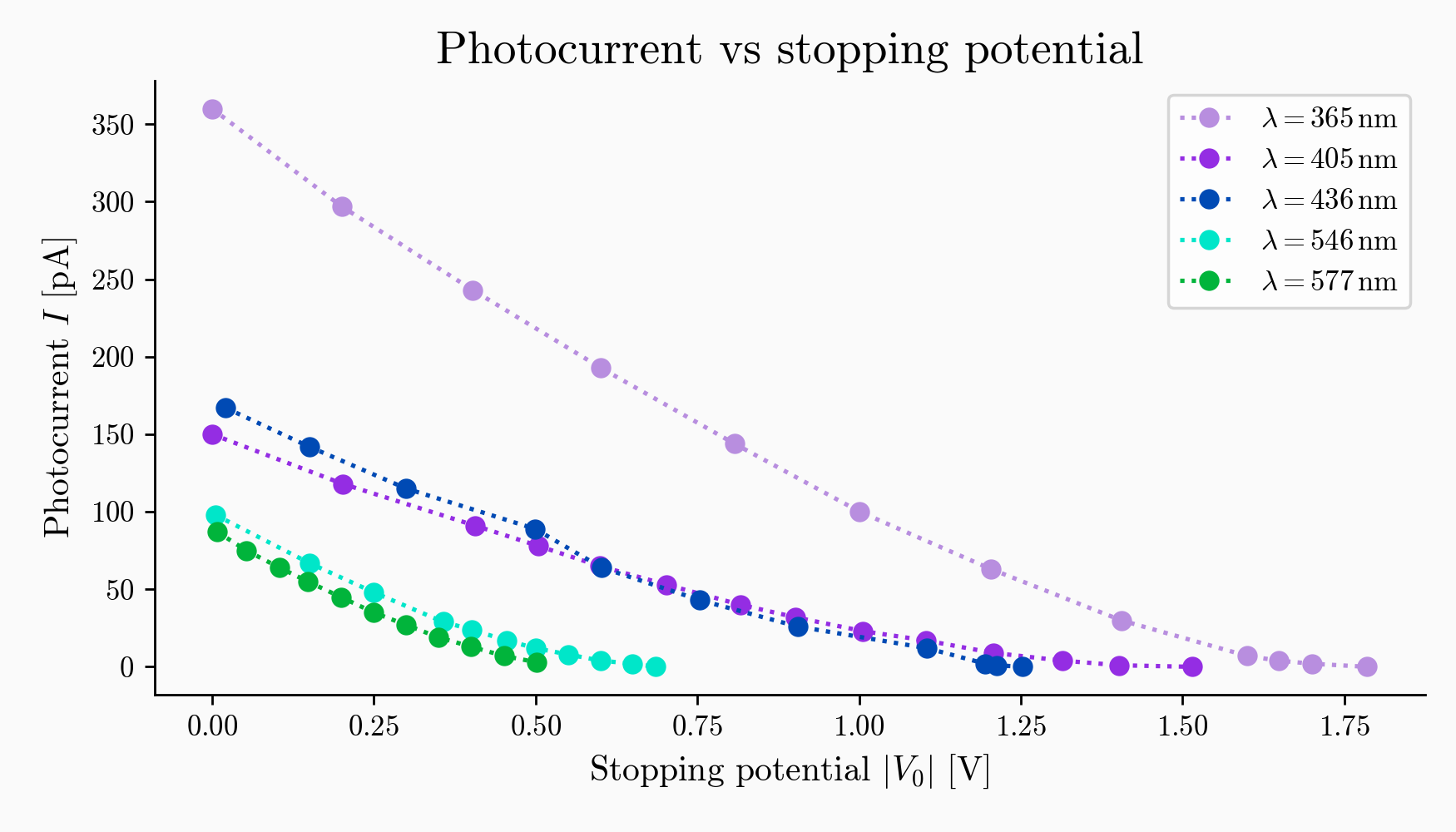
def plot_current_vs_stopping_potential():
    """
    Plots photocurrent through phototube as a function of the stopping
    potential between the phototube's anode and cathode at each incident photon
    frequency.
    """
    fig, ax = plt.subplots(figsize=(7, 4), facecolor="#fafafa")
    remove_spines(ax)
    ax.set_facecolor('#fafafa')
    ax.set_xlabel("Stopping potential $|V_0|$ [V]")
    ax.set_ylabel("Photocurrent $I$ [pA]")
    ax.set_title("Photocurrent vs stopping potential")

    for filename in sorted(os.listdir(data_dir)):
        if not filename.endswith(".csv"):
            continue  # skip non-CSV files

        # Extract wavelength form filename, e.g. "365.csv" becomes 365
        wavelength = int(filename.replace(".csv", ""))

        # Skip first row (which holds header text)
        data = np.loadtxt(data_dir + filename, delimiter=",", skiprows=1)

        # Extract potential and current from columns 0 and 1, respectively
        V = np.abs(data[:, 0])
        I = data[:, 1]
        
        ax.plot(V, I, linestyle=":", marker="o", color=colors[wavelength], 
                label="$\lambda = {} \, \mathrm{{nm}}$".format(wavelength))

    ax.legend()
    plt.tight_layout()
    plt.savefig(fig_dir + "current_vs_potential.png", format="png", dpi=250)
    plt.show()


def get_stopping_potentials():
    """
    Returns phototube stopping potential as a function of photon wavelength.
    These values are taken from the graphs in `current_vs_stopping_potential`;
    each stopping potential is the potential difference at which photocurrent
    falls to zero.
    """
    wavelength = 1e-9 * np.array([365, 405, 436, 546, 577])  # convert nm to m
    V = np.array([-1.785, -1.515, -1.252, -0.686, -0.501])
    return (wavelength, V)


def plot_stopping_potential_vs_frequency():
    """
    Plots the dependence of phototube stopping potential on photon frequency.
    """
    wavelength, V = get_stopping_potentials()
    V = np.abs(V)
    c = 3e8  # speed of light
    f = c / wavelength  # convert wavelength to frequency
    f /= 1e12  # convert Hz to THz

    fig, ax = plt.subplots(figsize=(7, 4), facecolor="#fafafa")
    remove_spines(ax)
    ax.set_facecolor('#fafafa')
    ax.set_xlabel("Photon frequency $f$ [THz]")
    ax.set_ylabel("Stopping potential $|V_0|$ [V]")
    ax.set_title("Stopping potential vs photon frequency")
    ax.plot(f, V, color=blue700, linestyle=":", marker="o")
    plt.tight_layout()
    plt.savefig(fig_dir + "potential_vs_frequency.png", format="png", dpi=250)
    plt.show()


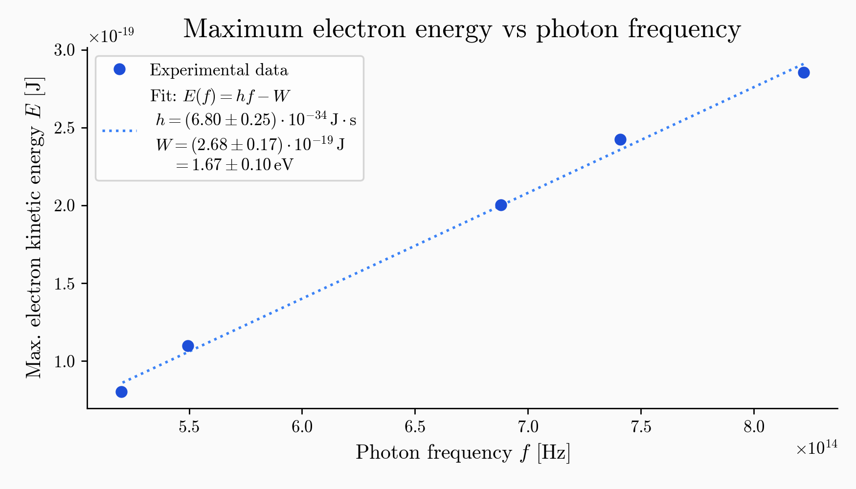
def analyze():
    """
    Estimates Planck's constant and the phototube cathode's work function from
    the dependence of maximum photoelectron kinetic energy on incident photon
    frequency.

    Maximum photoelectron kinetic energy $E_{max}$ and photon frequency $f$ are
    related by the equation
    [[
        E_{max}(f) = h*f - W,
    ]]
    where $W$ is the photocathode's work function and $h$ is Planck's constant. 
    At the stopping potential $V0$ when photocurrent falls to zero, 
    [[
        e0*|V0| = E_{max}
    ]],
    where e0 is the (positive) elementary charge.

    Steps:
        1. Use $V0$ and $e0$ to compute $E_{max}$
        2. Plot $E_{max}$ as a function of photon frequency $f$
        3. Use SciPy's curve_fit function to fit the experimental $E_{max}(f)$
           data to the linear model $E_{max}(f) = h*f - W$. The slope of the
           best-fit line is Planck's constant $h$ and the y-intercept is the
           photocathode's work function $W$.
    """
    wavelength, V0 = get_stopping_potentials()
    c = 3e8  # speed of light
    e0 = 1.6e-19
    f = c / wavelength  # convert wavelength to frequency
    E_max = np.abs(V0*e0)

    h_fit, W_fit, h_std, W_std = fit(f, E_max)

    f_fit = np.linspace(f[0], f[-1], 50)
    E_max_fit = E_max_model(f_fit, h_fit, W_fit)

    fig, ax = plt.subplots(figsize=(7, 4), facecolor="#fafafa")
    remove_spines(ax)
    ax.set_facecolor('#fafafa')
    ax.set_xlabel("Photon frequency $f$ [Hz]")
    ax.set_ylabel("Max. electron kinetic energy $E$ [J]")
    ax.set_title("Maximum electron energy vs photon frequency")

    # Plot experimental data
    ax.plot(f, E_max, linestyle="none", marker="o", color=blue700,
            label="Experimental data", zorder=10)

    # This chunk of code is just to make the scientific notation look
    # nice in the Matplotlib legend. It has only an aesthetic purpose.
    h_fit_exp, h_fit_man  = extract_exp_man(h_fit)
    h_std_exp, h_std_man  = extract_exp_man(h_std)
    W_fit_exp, W_fit_man  = extract_exp_man(W_fit)
    W_std_exp, W_std_man  = extract_exp_man(W_std)
    e0 = 1.6e-19  # elementary charge
    W_fit_eV = W_fit/e0
    W_std_eV = W_std/e0

    # Plot best-fit line and fit parameters; the code looks intimidating but is
    # really just a Python format string to create nice-looking scientific
    # notation in the Matplotlib legend
    ax.plot(f_fit, E_max_fit, linestyle=":", color=blue500, 
            label="Fit: $E(f) = h f - W$\n $h = ({:.2f} \pm {:.2f}) \cdot 10^{{{:d}}} \, \mathrm{{J}} \cdot \mathrm{{s}} $\n $W = ({:.2f} \pm {:.2f}) \cdot 10^{{{:d}}} \, \mathrm{{J}}$\n    $ = {:.2f} \pm {:.2f} \, \mathrm{{eV}}$".format(h_fit_man, float(h_std_man)/(10**(h_fit_exp - h_std_exp)), h_fit_exp, W_fit_man, float(W_std_man)/(10**(W_fit_exp - W_std_exp)), W_fit_exp, W_fit_eV, W_std_eV))

    ax.legend()
    plt.tight_layout()
    plt.savefig(fig_dir + "fit.png", format="png", dpi=250)
    plt.show()


def E_max_model(f, h, W):
    """
    A model, for use with SciPy's curve_fit function, to fit experimental data
    to the linear photoelectric effect relationship
    [[
        E_{max}(f) = h*f - W
    ]]
    between maximum photoelectron kinetic energy and photon frequency.

    Parameters
    ----------
    f : float
        Photon frequency
    h : float
        Experimental value of Planck's constant
    W : float
        Experimental value of photocathode's work function
    """
    return h*f - W


def fit(f, E_max):
    """
    Fits the inputted (f, E_max) data to the photoelectric effect equation
    [[
        E_{max}(f) = h*f - W
    ]]
    Outputs the best-fit values of the parameters $h$ and $W$ along with their
    standard errors.

    """
    popt, pcov = curve_fit(E_max_model, f, E_max)

    # Extract optimal parameter values
    h = popt[0]
    W = popt[1]

    # The standard errors of the fit parameters are the square roots of the
    # corresponding entries along the diagonal of the fit's covariance matrix
    h_std = pcov[0, 0]**0.5
    W_std = pcov[1, 1]**0.5

    return h, W, h_std, W_std


def extract_exp_man(float):
    """
    Extracts exponent and mantissa from the inputted floated number.
    For context see https://en.wikipedia.org/wiki/Floating-point_arithmetic
    Examples:
        - Input 6.626e-34 return (-34, 6.626)
        - Input -42e-1 returns (0, -4.2)
    """
    (sign, digits, exponent) = Decimal(float).as_tuple()
    exp = len(digits) + exponent - 1
    man = Decimal(float).scaleb(-exp).normalize()
    return exp, man


def remove_spines(ax):
    """
    Removes top and right spines from the inputted Matplotlib axis. This is for
    aesthetic purposes only and has no practical function.
    """
    ax.spines['top'].set_visible(False)
    ax.spines['right'].set_visible(False)
    ax.get_xaxis().tick_bottom()
    ax.get_yaxis().tick_left()


if __name__ == "__main__":
    plot_current_vs_stopping_potential()
    plot_stopping_potential_vs_frequency()
    analyze()